Blog Details | Academy Learning Club

The Mathematics Behind Artificial Intelligence

Engineer Duru
AI, Maths, Science
0 comment
29 Nov, 2025

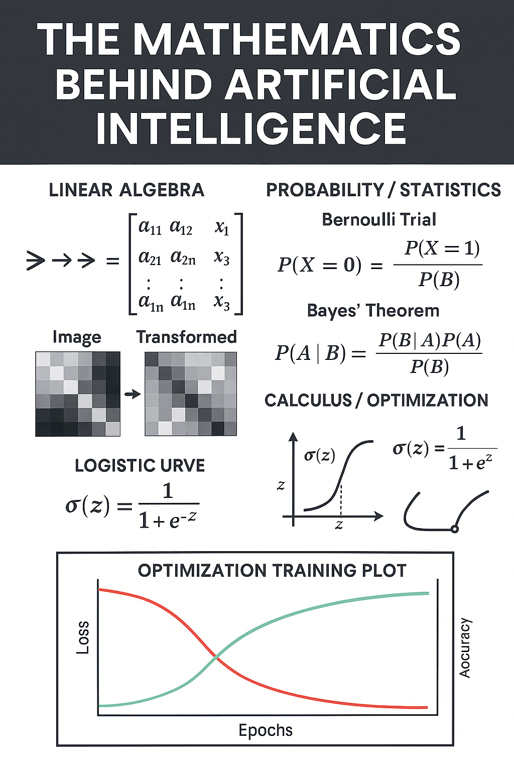
Artificial Intelligence (AI) often feels like magic. Machines recognize faces, translate languages, and even write poetry. But beneath the surface, AI is powered by something far more fundamental: mathematics. In this post, we’ll explore the three pillars of math that make AI possible—linear algebra, probability & statistics, and calculus & optimization—and even look at a Python simulation that brings these ideas to life.

Linear Algebra: Moving Data

At its core, AI is about numbers. Images, sounds, and words can all be represented as vectors and matrices—grids of numbers that capture information.

Matrix multiplication transforms data: rotate an image, compress a sound, or shift meaning in language.
Neural networks rely on these transformations to pass information forward, layer by layer.

Think of linear algebra as the engine that moves data through the AI pipeline.

Probability & Statistics: Guiding Decisions

AI doesn’t just move data—it makes decisions under uncertainty.

Probability distributions answer questions like: “What’s the chance this email is spam?”
Statistics help AI learn patterns from data, turning raw numbers into predictions.
Bayes’ theorem and logistic functions are the mathematical tools that allow AI to weigh evidence and update beliefs.

Probability is the compass that guides AI toward the most likely outcome.

Calculus & Optimization: Teaching Learning

AI learns by minimizing error. This is where calculus comes in.

Gradient descent is the process of rolling downhill toward the lowest error.
Each step adjusts the model’s weights, making predictions more accurate.
Over time, loss decreases while accuracy rises—a clear sign of learning.

Calculus is the teacher, showing AI how to improve with each iteration.

A Python Simulation of AI Math

To make this concrete, here’s a quick overview of a Python simulation built with SimPy and Matplotlib:

Producer: Generates synthetic data batches.
Linear Algebra Transform: Applies matrix operations to reshape data.
Probability Classification: Estimates outcomes with logistic scoring.
Trainer: Uses gradient descent to minimize error.
Plots: At the end, Matplotlib shows Loss vs Time and Accuracy vs Time.

The result? A mini AI factory where you can watch math in action—loss curves falling, accuracy curves rising.

import simpy
import numpy as np
import random
import matplotlib.pyplot as plt

# -----------------------------
# Config
# -----------------------------
RANDOM_SEED = 42
SIM_DURATION = 120.0
BATCH_INTERVAL = 4.0
BATCH_SIZE = 256
FEATURES = 32
LA_OP_TIME = 1.5
PROB_OP_TIME = 0.8
TRAIN_OP_TIME = 2.0
TRAIN_STEPS_PER_EPOCH = 5
EPOCHS = 3
CPU_CORES = 2
GPU_UNITS = 1

np.random.seed(RANDOM_SEED)
random.seed(RANDOM_SEED)

metrics_buffer = []  # Buffer for plotting

# -----------------------------
# Utility
# -----------------------------
def log(env, msg):
    print(f"[t={env.now:6.2f}s] {msg}")

# -----------------------------
# Data model
# -----------------------------
class DataBatch:
    def __init__(self, batch_id, x, y_true):
        self.id = batch_id
        self.x = x
        self.y_true = y_true
        self.x_transformed = None
        self.y_proba = None
        self.y_pred = None

# -----------------------------
# Pipeline processes
# -----------------------------
def producer(env, out_store):
    batch_id = 0
    while True:
        x = np.random.randn(BATCH_SIZE, FEATURES).astype(np.float32)
        w_true = np.random.randn(FEATURES).astype(np.float32)
        logits = x @ w_true + np.random.randn(BATCH_SIZE).astype(np.float32) * 0.5
        y_true = (1 / (1 + np.exp(-logits)) > 0.5).astype(np.int32)
        batch = DataBatch(batch_id, x, y_true)
        log(env, f"Batch {batch_id} arrived")
        yield out_store.put(batch)
        batch_id += 1
        yield env.timeout(BATCH_INTERVAL)

def linear_algebra_transform(env, gpu, in_store, out_store):
    W = np.random.randn(FEATURES, FEATURES).astype(np.float32) * 0.5
    b = np.random.randn(FEATURES).astype(np.float32) * 0.1
    while True:
        batch = yield in_store.get()
        with gpu.request() as req:
            yield req
            log(env, f"Batch {batch.id}: LA transform started")
            yield env.timeout(LA_OP_TIME)
            x_prime = batch.x @ W + b
            batch.x_transformed = np.maximum(x_prime, 0)
            log(env, f"Batch {batch.id}: LA transform done")
            yield out_store.put(batch)

def probability_classification(env, cpu, in_store, out_store):
    w_prob = np.random.randn(FEATURES).astype(np.float32)
    while True:
        batch = yield in_store.get()
        with cpu.request() as req:
            yield req
            log(env, f"Batch {batch.id}: Prob step started")
            yield env.timeout(PROB_OP_TIME)
            scores = batch.x_transformed @ w_prob
            proba = 1 / (1 + np.exp(-scores))
            batch.y_proba = proba
            batch.y_pred = (proba > 0.5).astype(np.int32)
            acc = (batch.y_pred == batch.y_true).mean()
            log(env, f"Batch {batch.id}: Prob step done (acc={acc:.3f})")
            yield out_store.put(batch)

def trainer(env, gpu, in_store):
    w_train = np.zeros(FEATURES, dtype=np.float32)
    lr = 0.05
    epoch = 0
    steps_in_epoch = 0
    while epoch < EPOCHS:
        batch = yield in_store.get()
        for step in range(TRAIN_STEPS_PER_EPOCH):
            with gpu.request() as req:
                yield req
                log(env, f"Batch {batch.id}: Training step {steps_in_epoch + 1} (epoch {epoch+1})")
                yield env.timeout(TRAIN_OP_TIME)
                scores = batch.x_transformed @ w_train
                p = 1 / (1 + np.exp(-scores))
                grad = (batch.x_transformed.T @ (p - batch.y_true)) / BATCH_SIZE
                w_train -= lr * grad
                loss = -(batch.y_true*np.log(np.clip(p,1e-8,1)) + (1-batch.y_true)*np.log(np.clip(1-p,1e-8,1))).mean()
                acc = ((p > 0.5).astype(np.int32) == batch.y_true).mean()
                metrics_buffer.append({
                    "t": env.now,
                    "epoch": epoch+1,
                    "step": steps_in_epoch+1,
                    "batch": batch.id,
                    "loss": float(loss),
                    "acc": float(acc)
                })
                log(env, f"Batch {batch.id}: Training done (loss={loss:.4f}, acc={acc:.3f})")
                steps_in_epoch += 1
        if steps_in_epoch >= TRAIN_STEPS_PER_EPOCH:
            epoch += 1
            steps_in_epoch = 0
            log(env, f"Epoch {epoch} completed")

def sink(env, in_store):
    while True:
        batch = yield in_store.get()
        log(env, f"Batch {batch.id}: Pipeline complete")

# -----------------------------
# Setup
# -----------------------------
def setup(env):
    cpu = simpy.Resource(env, capacity=CPU_CORES)
    gpu = simpy.Resource(env, capacity=GPU_UNITS)
    q_incoming = simpy.Store(env)
    q_after_la = simpy.Store(env)
    q_after_prob = simpy.Store(env)
    env.process(producer(env, q_incoming))
    env.process(linear_algebra_transform(env, gpu, q_incoming, q_after_la))
    env.process(probability_classification(env, cpu, q_after_la, q_after_prob))
    env.process(trainer(env, gpu, q_after_prob))
    env.process(sink(env, q_after_prob))

# -----------------------------
# Main
# -----------------------------
if __name__ == "__main__":
    env = simpy.Environment()
    setup(env)
    log(env, "Simulation started")
    env.run(until=SIM_DURATION)
    log(env, "Simulation finished")

    # Plotting
    times = [m['t'] for m in metrics_buffer]
    losses = [m['loss'] for m in metrics_buffer]
    accuracies = [m['acc'] for m in metrics_buffer]

    plt.figure(figsize=(10,5))
    plt.plot(times, losses, marker='o', color='red', label='Loss')
    plt.title("Loss vs Time")
    plt.xlabel("Simulation Time (s)")
    plt.ylabel("Loss")
    plt.grid(True)
    plt.legend()
    plt.show()

    plt.figure(figsize=(10,5))
    plt.plot(times, accuracies, marker='x', color='blue', label='Accuracy')
    plt.title("Accuracy vs Time")
    plt.xlabel("Simulation Time (s)")
    plt.ylabel("Accuracy")
    plt.ylim(0,1)
    plt.grid(True)
    plt.legend()
    plt.show()

Faith + Tech Reflection

Just as Proverbs reminds us, “By wisdom a house is built” (Proverbs 24:3). AI, too, is built on unseen foundations—mathematics. Whether in faith or technology, the invisible structures are what make everything else possible.

Conclusion

AI isn’t magic—it’s math.

Linear algebra moves data.
Probability guides decisions.
Calculus teaches learning.

If you want to understand AI, start with the math. It’s the true code of intelligence.

AI, Maths, Science